Pharmacodynamics is the study of how drugs have effects on the body. The most common mechanism is by the interaction of the drug with tissue receptors located either in cell membranes or in the intracellular fluid. The extent of receptor activation, and the subsequent biological response, is related to the concentration of the activating drug (the ‘agonist’). This relationship is described by the dose–response curve, which plots the drug dose (or concentration) against its effect. This important pharmacodynamic relationship can be influenced by patient factors (e.g. age, disease) and by the presence of other drugs that compete for binding at the same receptor (e.g. receptor ‘antagonists’). Some drugs acting at the same receptor (or tissue) differ in the magnitude of the biological responses that they can achieve (i.e. their ‘efficacy’) and the amount of the drug required to achieve a response (i.e. their ‘potency’). Drug receptors can be classified on the basis of their selective response to different drugs. Constant exposure of receptors or body systems to drugs sometimes leads to a reduced response (i.e. ‘desensitization’).
Introduction to the dose-response relationship
When the relation between drug dose (X-axis) and drug response (Y-axis) is plotted on a base 10 logarithmic scale, this produces a sigmoidal dose–response curve (Fig A). This representation is more useful than a linear plot because it expands the dose scale in the region where drug response is changing rapidly and compresses the scale at higher doses where large changes have little effect on response. Clinical responses that might be plotted in this way include change in heart rate, blood pressure, gastric pH or blood glucose, as well as more subtle phenomena such as enzyme activity, accumulation of an intracellular second messenger, membrane potential, secretion of a hormone, or contraction of a muscle.
Progressive increases in drug dose produce increasing drug effects, but these occur over a relatively narrow part of the overall concentration range; further increases in drug dose (or concentration) beyond this range produce little extra effect. The clinical implication of this relationship is that simply increasing drug dose may not result in any further beneficial effects for patients and may cause adverse effects. The maximum response on the curve is referred to as the Emax and the dose (or concentration) producing half this value (Emax/2) is the ED50 (or EC50). The effective dose range can be considered as spanning the straight-line segment of the log dose–response curve (corresponding to 20–80% of Emax). The maximum tolerated dose is the highest dose of a drug that can be administered without the development of dose-related adverse effects.
The addition of a competitive antagonist to an agonist will lead to a shift in the agonist dose–response curve to the right because higher agonist concentrations are now required to achieve a given percentage receptor occupancy (and therefore effect) (Fig B). Dose–response curves of the agonist constructed in the presence of increasing doses of a competitive antagonist are progressively shifted to the right. Nevertheless, the effect of a reversible competitive antagonist can always be overcome by giving the agonist at a sufficiently high concentration (i.e. it is surmountable). Many clinically useful drugs are competitive antagonists (e.g. atenolol, naloxone, atropine, cimetidine). Non-competitive antagonists inhibit the effect of an agonist in ways other than direct competition for receptor binding with the agonist (e.g. by affecting the secondary messenger system). This makes it impossible to achieve maximum response even at very high agonist concentration. At a given concentration, non-competitive antagonists not only shift the agonist dose–response curve to the right but also decrease the Emax (Fig C). Irreversible antagonists can be considered as a particular form of non-competitive antagonist characterized by antagonism that persists, even after the antagonist has been removed. Common examples are aspirin and omeprazole. This form of antagonism disappears only when new proteins or enzyme are synthesized. This explains why aspirin is effective, even when taken intermittently, as prophylaxis against cardiovascular events.
The dose-response relationship to the same drug varies between individuals because of various factors, such as differences in receptor number and structure, receptor-coupling mechanisms and physiological changes resulting from differences in genetics, age and health. For example, the effect of the loop diuretic, furosemide, is often significantly reduced at a given dose in patients with renal impairment. A further source of variability is that the same dose of drug does not achieve the same tissue drug concentrations in all individuals because of differences in handling (e.g. metabolism, excretion). In reality, it is this pharmacokinetic variation that explains most of inter-individual variation in drug response seen in clinical practice.
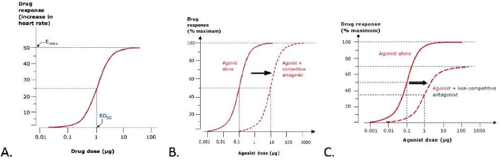
Figure. Dose–response curves. A. Basic features. B. The effect of co-administering an agonist with a competitive antagonist. C. The effect of administering an agonist with a non-competitive antagonist. (Note that, in reality, it is ligand concentration (and resulting receptor occupation) that affects response. When discussing ‘the dose– response curve’ it is often assumed that the drug dose and ligand concentration are closely linked. This is likely to be the case during an in vitro pharmacological experiment but the relation between an ingested drug dose and relevant tissue concentration in a human can be more complex.)
RESOURCES
Receptor Affinity
Affinity of ligands is a function of both the rate of association and the rate of dissociation of the ligand–receptor complex; the former depends on the ‘goodness of fit’ at a molecular level, whereas the latter depends on how tightly the ligand is bound (the strength of the chemical bond). Systems requiring rapid fine modulation (e.g. nerve synapses) must have agonists with a low receptor affinity because those with high receptor affinity would produce unnecessarily prolonged responses. During stimulation, agonist concentration near the receptor must be relatively high, but the agonist is then cleared rapidly by active transport. In contrast, growth factors are typically peptides with very high affinity for their receptors, and achieve their effects at concentrations that are difficult to detect in vivo. Some drug–receptor interactions are so strong that they are effectively irreversible. A good example is aspirin, which irreversibly inhibits its target, the enzyme cyclooxygenase.
RESOURCES
Agonist affinity can be measured in terms of a dissociation constant for agonist binding to a receptor using ligand binding or functional assays. In such systems, however, measurements of affinity are contaminated by efficacy. In this 11-page review, the author describes methods to assess affinity and efficacy at G protein-coupled receptors using experimental approaches to separate the two parameters. This article would be appropriate for a student in pharmacology who has extensive knowledge of receptor theory and G protein-coupled receptors.
 | Cellular receptors: Part 2, binding, affinity, selectivity, potency
This 8 minute animated YouTube video by PharmacoPhoto provides a succinct description of the molecular interactions between receptors and their ligands. It is suitable for intermediate level learners.
Receptor selectivity
Receptors are named on the basis of their major endogenous agonist (e.g. adrenergic, serotoninergic, opioid). They are then usually ‘sub-‐typed’ on the basis of their selectivity for agonists or antagonists. Agonist selectivity is determined by the ratio of EC50 of the dose– response curve at the two different receptor subtypes. For example, β-‐adrenoceptors can be sub-‐typed into β1 and β2, on the basis of their responsiveness to the endogenous agonist, noradrenaline. The concentration required to cause bronchodilatation (via β2 adrenoceptors) is ten times higher than that required to cause tachycardia (via β1 adrenoceptors). Receptor sub-‐ types can also be distinguished by the relative effectiveness of drugs that antagonize the effects of their full agonist, measured as the relative shift of the agonist dose–response curves achieved by a single dose of antagonist affecting responses mediated through the two receptors. It is important for prescribers to remember that selectivity for a receptor subtype is only a relative concept (i.e. selectivity does not equate with specificity). Agonist or antagonist drugs that are considered to be ‘selective’ for one receptor subtype can still produce significant effects at other subtypes if a high enough dose is given. This is particularly important if one receptor subtype activates the beneficial effects while another activates the adverse effects. For instance, ‘cardioselective’ β-‐adrenoceptor blocking drugs have anti-‐anginal effects on the heart (β1) but may cause bronchospasm in the lung (β2) and are absolutely contraindicated for asthmatic patients. Selectivity is useful in clinical practice only when the ratio of the impact of the drug at the two receptor sites is 100 or more. When selectivity is lower, it is difficult to predict drug doses that will exploit the difference in subtype activity.
RESOURCES
The term selectivity is use to describe the ability of a drug to affect a particular gene, protein, signaling pathway, etc. in preference to others. In the search for new therapeutic agents, selectivity is thought to have a high degree of desirability. The single target reasoning for therapeutic development may be flawed, however, in that there may be a balance and interplay of multiple signaling networks which could result in unintended consequences. In this debate article, the authors describe specific examples in discussing the issues related to drug selectivity. This 7-page article would be appropriate for advanced students in pharmacology who have a thorough understanding of pharmacodynamics.
Receptor selectivity
Efficacy is the term used to describe the extent to which a drug can produce a response when all available receptors or binding sites are occupied (i.e. Emax on the dose–response curve). When comparing drugs acting at the same receptor, a full agonist will have the greatest efficacy and can produce the maximum response of which the receptor is capable. A partial agonist at the same receptor, by definition, will have a lower efficacy, even when all receptor sites are occupied. The concept of efficacy is not restricted to comparing the effects of drugs that act at the same receptor. The term therapeutic efficacy is used to describe the comparison of drugs that produce the same therapeutic effects on a biological system but do so via different pharmacological mechanisms (e.g. loop and thiazide diuretics, proton pump inhibitors and H2- antagonists). Potency is a term used to describe the amount of a drug required for a given response. More potent drugs produce biological effects at lower doses (or concentrations), which means that they have a lower ED50 (Fig)
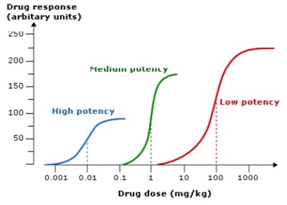
Figure. Dose response curves for drugs with high, medium and low potency acting on the same target. Note that the drug with the highest potency has the lowest efficacy and vice versa.
The potency of a drug is related to its affinity for the receptor (i.e. how readily the drug-receptor complex is formed). Less potent drugs can have an efficacy similar to that of a more potent one; the difference in potency can be readily overcome by giving the less potent drug in higher doses. This is illustrated by the varying recommended dose ranges of drugs acting at the same drug target (e.g. H2 antagonists, ACE inhibitors).
When choosing between drugs with a similar beneficial effects (e.g. analgesia) from a group of similar drugs it might seem logical to choose the one with the greatest therapeutic efficacy. However, in some cases the most efficacious drug may be less favorable because the same mechanism of action that leads to clinical benefits may also be responsible for causing dose-limiting adverse-effects (e.g. opioids, β1-adrenoceptor blocking drugs). When the same action leads to both beneficial and adverse effects, the latter can be minimized by carefully increasing (titrating) the dose. However, some drugs have a steeper dose–response curve, which makes it more difficult to titrate to the dose that is effective but avoids adverse effects.
The potency of a drug is rarely a reason for choosing one out of a collection of drugs with similar beneficial therapeutic effects. This is because any differences in potency can be overcome simply by giving higher doses. Although differences in relative potency can be overcome by altered dosage, it should be remembered that most of the adverse effects of drugs are also dose-related. Potency may be relevant if these occur by a mechanism other than the receptor–ligand interaction that mediates the beneficial effect (because only the more potent drug will be active at concentrations that avoid unwanted adverse effects).
For these reasons greater potency or efficacy does not necessarily mean that one drug is preferable to another. When judging the relative merits of drugs for a patient, prescribers should also consider other important factors, such as the overall adverse effect profile, therapeutic index, ease of administration for the patient, duration of effect (i.e. the number of doses needed each day) and cost.
RESOURCES
These are the second and third in a series of 4 simulations related to dose-response relationships. These two simulations focus on potency and efficacy. In the first simulation the learner can vary the potency by the use of a slider and observe the effects on the log dose-response curve. The second simulation allows the learner to vary the efficacy and observe the changes. This is a more kinesthetic approach to illustrating these concepts in that it allows the learner to experiment. Although targeted for early learners in pharmacology, students should have a basic understanding of the concepts before using the simulation.
Therapeutic index
When drugs are used in clinical practice, the prescriber is unable to construct a careful dose–response curve for each individual patient. Therefore, most drugs are licensed for use within a recommended dose range that is expected to be close to the top of the dose–response curve for most patients. This ensures that most patients will achieve a good clinical response without the need for frequent review and dose increases. However, this means that it is sometimes possible to achieve the desired therapeutic response at doses towards the lower end of the recommended range (or below).
The adverse effects of drugs are often dose-related in a similar way to the beneficial effects. It is possible to construct a dose-response curve for these adverse effects in the same way as shown for the beneficial effects, with higher doses usually required to cause the adverse effect. The ED50 points for each curve in the Figure indicate that the ratio between the doses that have similar proportionate effects on the two outcomes is 10/0.1 = 100. This ratio is known as the ‘therapeutic index’. In reality, drugs have multiple potential adverse effects but the concept of therapeutic index is usually reserved for those requiring dose reduction or discontinuation. For most drugs, the therapeutic index is greater than 100 but there are some notable exceptions with therapeutic indices less than 10, which are in common use (e.g. digoxin, warfarin, insulin, phenytoin, opioids). Drugs with low therapeutic indices are more difficult to prescribe and hazardous for patients but they are still preferred if there are no alternative drugs with similar efficacy (e.g. anti-cancer drugs). The doses of such drugs have to be titrated carefully for individual patients to maximize benefits but avoid adverse effects. This is done by monitoring drug effects, either clinically or using regular blood tests (often known as ‘therapeutic drug monitoring’).
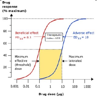
Figure. Dose–response curves for the beneficial and adverse effects of a drug. Prescribers will aim to prescribe doses that maximize benefits and minimize harms, which is easier for drugs where the ratio between the dose causing harm and that causing benefit (the ’therapeutic index’) is high.
RESOURCES
Dose-response curves and therapeutic index
In addition to providing definitions of terms for the learner (threshold, potency, efficacy) there is a description of how graded and quantal dose-response curves are obtained and the information which can be derived from each. A discussion of therapeutic index is included in relation to drug safety. This is appropriate for an early learner in pharmacology.
This is the fourth in a series of 4 simulations related to dose-response relationships. This simulation focuses on therapeutic index. In this simulation the learner can vary the therapeutic index by the use of a slider and observe the effects on the relative positions of the dose-response curves for the desired and adverse effects. This is a more kinesthetic approach to illustrating these concepts in that it allows the learner to experiment. Although targeted for early learners in pharmacology, students should have a basic understanding of the concepts before using the simulation.
This approximately 400-word essay describes the equation for therapeutic index together with easily understandable descriptions for how the ED50 and TD50 are determined from quantal dose-response relationships. Several examples of drugs with a narrow therapeutic index are provided at the end. This is appropriate for an early learner in pharmacology but they should have an understanding of dose-response relationships before viewing this resource.
This 350-word essay briefly describes the characteristics of a log dose-response curve and information that can be discerned when comparing dose-response curves. Each is accompanied by a figure. This is an easy to understand description of dose-response curves.
This is an almost 60 minute lecture on the general principles of pharmacology. The first half deals with drugs, pH and pKa including the Henderson-Hasselbalch equation. The latter portion of the presentation (about the last 15 minutes) focuses on dose-response relationships including graded and quantal with a discussion of potency and efficacy. This is appropriate for a beginning student in pharmacology.
This is a 30 minute video which provides a short overview of the relationship between drug dose and response. It covers the graphical representation of dose-response or concentration-effect relationships, and defines terms including affinity, efficacy, potency and partial agonist. This is appropriate for an early learner in pharmacology.